Creates a psitbxdcd object containing the description of the geometry of the chords of a diagnostic.
dcd = psitbxdcd(rd,zd,phid,pvd,tvd,nd,t)
The function psitbxdcd is used to create a psitbxdcd object that contains the description of the geometry of the chords of a diagnostic. The fields of a psitbxdcd object and the corresponding input arguments have the following meaning:
The size of rd,zd,phid,pvd,tvd follows the following rules:
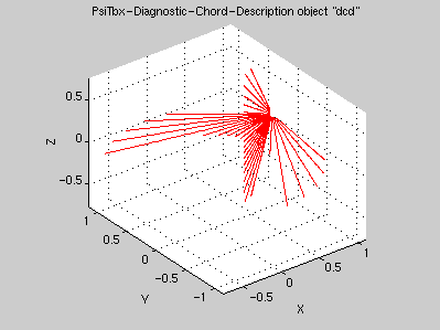
Here is an example with two cameras with 20 detectors each, the first one with a poloidal coverage, the second one with a toroidal coverage:
rd = 1.2;
zd = 0;
phid = pi/8;
pvd = [linspace(-pi/3,pi/3,20);zeros(1,20)];
tvd = [zeros(1,20);linspace(-pi/3,pi/3,20)];
dcd = psitbxdcd(rd,zd,phid,pvd,tvd)
 dcd is a PsiTbx-Diagnostic-Chord-Description object =
      rd: [2x20 double]
      zd: [2x20 double]
    phid: [2x20 double]
     pvd: [2x20 double]
     tvd: [2x20 double]
      nd: 81
       t: []
plot(dcd)
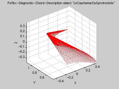
The possibility to have real-time scaning diagnostic is included. In that case the last dimension of the fields of the psitbxdcd object represents the time base. Given as an example Le cauchemar du gyrotroniste:
td = linspace(0,1,73);
rd = 1.2;
zd = 0;
phid = pi/2;
pvd = pi/6*cos(pi*td);
tvd = pi/6*sin(2*pi*td);
LeCauchemarDuGyrotroniste = psitbxdcd(rd,zd,phid,pvd,tvd,[],td);
plot(LeCauchemarDuGyrotroniste)
Computes the intersection between diagnostic chords described by a psitbxdcd object and a cylindrical coordinate grid contained in a psitbxgrid object.
s = intersect(dcd,g)
The method intersect applies to a psitbxdcd object and computes the intersection between the chords and a grid in cylindrical coordinates. It returns an array of linear coordinates along the chords of size [dcd.nd,size(dcd)]. The main purpose of intersect is to provide the coordinate of the points for building a psitbxgrid object of type 'Diagnostic-Chords'.
For those chords who do not cross the domain of the grid, NaN's are returned. For those chords who cross the domain twice, the first segment is considered.
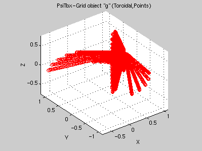
dcd = psitbxdcd('Demo');
s = intersect(dcd,psitbxgrid('Cylindrical','Grid','Default'));
gdc = psitbxgrid('Diagnostic-Chords','Points',{s},dcd)
 gdc is a PsiTbx-Grid object =
       type: 'Diagnostic-Chords'
      label: {1x1 cell  }
    storage: 'Points'
          x: {1x1 cell  }
          t: []
        par: [1x1 struct]
        csp: [1x1 struct]
Only awfull calculation of intersections between lines, planes and cylinders using analytical geometry.
Creates a psitbxfun object containing a function defined on a spatial grid.
 f = psitbxfun(x,g)

 f = psitbxfun(x,g,t)
The function psitbxfun is used to create a psitbxfun object that contains a function defined on a spatial grid. If this function does not depend on time, psitbxfun(x,g) is used with x containing the function value(s) defined on the psitbxgrid g. If the function varies in time, use the form psitbxfun(x,g,t).
The size of the matrix x must be [size(g)[,n1,...][,nt]]. The optional dimension n1,... can be used for multi-value functions (for example the wave length for spectroscopic measurements). If the time argument is given, then the last dimension of x, nt must correspond to length(t).
For degenerated coordinates, that have a size of one, the following rules apply:
Singleton dimension in x arising from degenerated coordinates can be omitted.
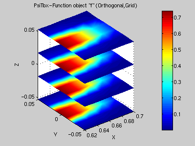
A fairly simple function defined on a cylindrical coordinate grid:
rzphi = {0.62:.02:0.7,-.05:.02:.05,pi/180*(-3:2:3)};
g = psitbxgrid('Orthogonal','Grid',rzphi);
[rzphi{:}] = ndgrid(rzphi{:});
x = exp(-300*(rzphi{1} - g.x{1}(1)).^2) .* exp(-3000*rzphi{2}.^2);
f = psitbxfun(x,g)
 f is a PsiTbx-Function object =
       x: [5x6x4 double    ]
    grid: [5x6x4 psitbxgrid]
       t: []
plot(f)
A very common concept in Tokamak physics is the profile, that is a quantity constant on a flux surface and therefore depending only on the flux coordinate. Such a profile is trivialy represented by a function on a 1-D grid, here the canonical parabolic profile:
g = psitbxgrid('Flux','Grid',{linspace(0,1,41),NaN,NaN});
f = psitbxfun(1-linspace(0,1,41)'.^2,g)
 f is a PsiTbx-Function object =
       x: [41x1   double    ]
    grid: [41x1x1 psitbxgrid]
       t: []
plot(f)
Method to compute the indefinite integral of a psitbxfun object over spatial coordinates
 f = cumsum(f,dim)

 f = cumsum(f,dim,'metric')
The method cumsum applies on a psitbxfun object defined on grid with 'Grid' storage and returns a psitbxfun containing its indefinite integral along the specified dimensions dim. For example if dim = 1, the integral is performed along the first coordinate, if dim = [2,3], the surface integral along coordinates 2 and 3 is returned, if dim = [1,2,3], the volume integral is returned.
By specifying the option 'metric', the appropriate metric will be taken into account; simply the function f.*metric(f.grid,dim) is integrated.
Uses a trapeze integration.
Method to average a psitbxfun object over spatial coordinates
 f = mean(f,dim)

 f = mean(f,dim,w)

 f = mean(f,dim,'metric')

 f = mean(f,dim,w,'metric')
The method mean applies on a psitbxfun object defined on grid with 'Grid' storage and returns a psitbxfun containing the function averaged along the specified dimensions dim. For example if dim = 1, the average is performed along the first coordinate, if dim = [2,3], the surface average along coordinates 2 and 3 is returned, if dim = [1,2,3], the volume average is returned.
Note that the grid on which the returned function is defined will become degenerated in the dimension along which average is carried out.
In the call mean(f,dim,w), w is a psitbxfun object playing the role of a weight in the average.
By specifying the option 'metric', the appropriate metric will be taken into account; simply the function f.*metric(f.grid,dim) is average.
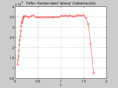
Average plasma current density
jphi = psitbxtcv(10000,'JPHI');
jphiavg = mean(jphi,[1,2],'metric');
plot(jphiavg)
Method to interpolate a psitbxfun object on a specified grid.
 f2 = psitbxf2f(f,g2)

 f2 = psitbxf2f(f,g2,der)

 f2 = psitbxf2f(f,der)
The method psitbxf2f applies on a psitbxfun object to interpolate the embended function on new space points. In the call psitbxf2f(f,g2) the psitbxfun object represents a function defined on a psitbxgrid which must have 'Grid' storage. g2 is a psitbxgrid object specifying the new space points on which the function f must be interpolated. Those can be given in any coordinate systems. Points outside the definition domain of the function will be assigned a NaN. If any coordinate of g2 is a NaN, which means that any function defined on g2 is independant of this coordinate, then the function f must also be independant along the corresponding coordinate.
The optional argument der is a three element vector that specifies the spatial derivative order to apply along each spatial coordinate. Note that since functions are interpolated with cubic spline, any order bigger than 3 will results in a zero function.
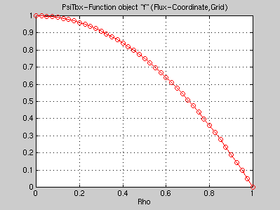
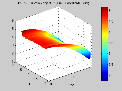
How to compute the normalised flux coordinate along diagnostic chords:
dcd = psitbxdcd('Demo');
psi = psitbxtcv(10000,.5,'01');
gdc = psitbxgrid('Diagnostic-Chords','Points',{intersect(dcd,psi.grid)},dcd);
rho = sqrt(psitbxf2f(psi,gdc));
plot(rho)
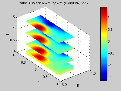
How to compute the radial derivative of the poloidal flux which is related to the vertical magnetic field:
psi = psitbxtcv(10000);
dpsidz = psitbxf2f(psi,[1,0,0]);
plot(dpsidz)
In a first step the points of g2 where the function f must be interpolated are transformed to compute their coordinates in the coordinate system on which the function f is defined, using the method psitbxg2g. Then the function f is interpolated in each spatial direction with cubic splines. The edge conditions are Not-A-Knot conditions except along angular coordinates which span 2×pi, in which case periodic edge conditions are used. Finaly this cubic spline interpolant is evaluated at the new positions, to the appropriate derivative order.
Note that interpolation requires the function to be smooth. For example interpolating the square-root of the poloidal flux defined in cylindrical coordinates yields problem on the magnetic axis where its first derivative is not continuous.
Method to integrate a psitbxfun object over spatial coordinates
 f = sum(f,dim)

 f = sum(f,dim,'metric')
The method sum applies on a psitbxfun object defined on grid with 'Grid' storage and returns a psitbxfun containing the function integrated along the specified dimensions dim. For example if dim = 1, the integral is performed along the first coordinate, if dim = [2,3], the surface integral along coordinates 2 and 3 is returned, if dim = [1,2,3], the volume integral is returned.
Note that the grid on which the returned function is defined will become degenerated in the dimension along which integration is carried out.
By specifying the option 'metric', the appropriate metric will be taken into account; simply the function f.*metric(f.grid,dim) is integrated.
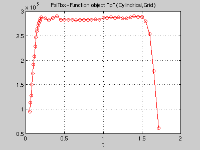
A non trivial way to compute the plasma current
jphi = psitbxtcv(10000,'JPHI');
ip = sum(jphi,[1,2]);
plot(ip)
Uses a trapeze integration.
Methods for mathematical operations on psitbxfun objects
 f = f + a

 f = f + g

 f = f .* a

 f = sqrt(f)

 f = f > 0
Most of the mathematical operators and functions have been overloaded for psitbxfun objects. For multi operand functions, the following rules apply:
Express the current density in MA/m2
jphi = psitbxtcv(10000,'JPHI')/1e6;
Creates a psitbxgrid object containing the definition of a spatial grid
g = psitbxgrid(type,storage,x[,p1,...])
The function psitbxgrid is used to create a psitbxgrid object that contains the description of a spatial grid. The usual call is psitbxgrid(type,storage,x).
The character argument type specifies which coordinate system is used. Possible choices are:
The character argument storage specifies the way the grid points are stored in the x field of the psitbxgrid object. This field and argument is a cell array containing three double arrays. Possible values for storage are:
For 1-D or 2-D grids, the corresponding array in x can be replaced either by a constant, for example for things that lie entirely on a plane, or by a single NaN which means that the problem does not depend on this particular coordinate. A grid can also be extended to other dimension that the basic space and time coordinates. For example a fourth dimension can be added that would represents a frequency or a wave length if necessary.
There are some combinations of type and storage for which the x argument can be given as the string 'Default', which will returns a predefined grid, in particular psitbxgrid('Flux-Coordinate','Grid','Default')
For its points to be absolutely positioned in space, some coordinate systems requires additional information. Such an information is given in a list of optional arguments to the function psitbxgrid. Here is a list of these pieces of information:
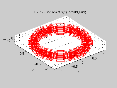
A 'Toroidal' grid with 'Grid' storage
x = {linspace(0,.2,6),linspace(-pi,pi,7),linspace(0,2*pi,25)};
r0z0 = {1,0};
g = psitbxgrid('Toroidal','Grid',x,r0z0)
 g is a PsiTbx-Grid object =
       type: 'Toroidal'
      label: {1x3 cell  }
    storage: 'Grid'
          x: {1x3 cell  }
          t: []
        par: [1x1 struct]
        csp: [1x1 struct]
plot(g)
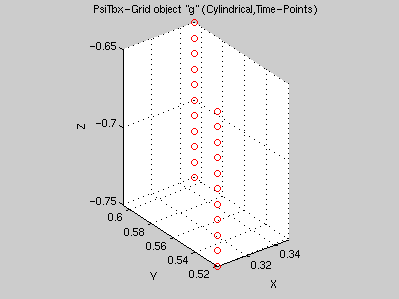
Two probes moving along the Z direction
t = linspace(0,.1,11);
x = {repmat([.6;.7],1,11),[t;t]-.75,pi/3};
g = psitbxgrid('Cylindrical','Time-Points',x,t)
 g is a PsiTbx-Grid object =
       type: 'Cylindrical'
      label: {1x3  cell  }
    storage: 'Time-Points'
          x: {1x3  cell  }
          t: [1x11 double]
        par: [1x1  struct]
        csp: [1x1  struct]
plot(g)
Method to compute the metric of a psitbxgrid object
f = metric(g,dim)
The method metric applies on a psitbxgrid object with 'Grid' storage and returns a psitbxfun containing the metric along the specified dimensions dim. For example if dim = 1, the metric along the first coordinate is returned, if dim = [2,3], the metric of the surface element along coordinates 2 and 3 is returned, if dim = [1,2,3], the volume element is returned. In addition if dim is negative, the norm of the gradient of the specified coordinate is returned.
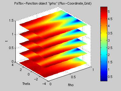
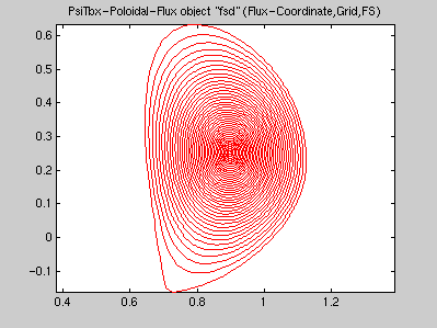
The very important gradient of rho entering the expression of the SEF (Shape Enhancement Factor)
fsd = psitbxtcv(10000,'FS');
grho = metric(fsd,-1);
plot(grho)
For the flux-coordinate system, the metric matrix is not diagonal; for the others it is trivial. Here are the formulae:

Method to transform a psitbxgrid object on a different coordinate system
 g2 = psitbxg2g(g,type)

 g2 = psitbxg2g(g,type,p1,...)
The method psitbxg2g applies on a psitbxgrid object to transform the coordinates of its points in a new coordinate system. In the call psitbxg2g(g,type), g is a psitbxgrid object and type a character string that specifies the new coordinate system; it can take the value of the type argument of the psitbxgrid function. psitbxg2g returns a psitbxgrid object with the same spatial points but with coordinates expressed in the new system.
Note that the storage may be altered; in particular 'Grid' storage may be transformed in 'Points' or 'Time-Points' storage because points in the new system do not align on a grid anymore.
It is impossible to map points on a 'Diagnostic-Chords' system, since this system is discrete in space.
Some transformations require additional information that will be sought in the par field of the g argument or in additional optional arguments, following the same rules as for the psitbxgrid function. These transformations are:
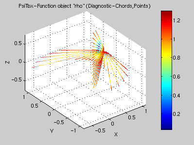
Position of the chord points in toroidal coordinates:
dcd = psitbxdcd('Demo');
s = intersect(dcd,psitbxgrid('Cylindrical','Grid','Default'));
gdc = psitbxgrid('Diagnostic-Chords','Points',{s},dcd);
g = psitbxg2g(gdc,'Toroidal',{.89,0});
plot(g)
There are a set of basic transformations defined. All the others are composed from the basic set, which is:

Creates a psitbxpsi object containing the poloidal flux description or the flux surface description.
psi = psitbxpsi(x,grid,t,form)
psi = psitbxpsi(x,grid,t,form,rmag,zmag)
psi = psitbxpsi(x,grid,t,form,rmag,zmag,iter,tol)
The function psitbxpsi is used to create a psitbxpsi object, which is a child of the psitbxfun class that contains either the poloidal flux in cylindrical coordinates or the flux surface contours in toroidal coordinates. In the call psitbxpsi(x,grid,t,form) depending on the form argument:
Optional arguments allows to specify the position of the magnetic axis rmag and zmag and convergence parameters for the method psitbxp2p, iter and tol.
Method to compute geometrical quantities from a psitbxpsi object
fsg = psitbxfsg(fsd)
The method psitbxfsg applies on a psitbxpsi object with format 'FS' and returns a structure with fields of class psitbxfun:
fsd = psitbxtcv(10000,'FS');
fsg = psitbxfsg(fsd);
plot(fsg.grho)
Uses the following definitions:
Method to change the format of a psitbxpsi object
 psi = psitbxp2p(psi,'01')

 fsd = psitbxp2p(psi,'FS')

 fsd = psitbxp2p(psi,'FS',g)
The method psitbxp2p applies on a psitbxpsi object and returns a psitbxpsi object with the specified form:
psi = psitbxtcv(10000,.5);
fsd = psitbxp2p(psi,'FS');
plot(fsd)
Uses Gauss-Newton iterations to locate either the maximum or the contour level. Iteration convergence is controlled by the iter and tol fields of the psitbxpsi object.
Easy access to quantities relevant for the Psi-Toolbox directly from the TCV shot files
psitbxtcv(shot,form)
psitbxtcv(shot,time,form)
The function psitbxtcv builds object compatible with the Psi-Toolbox from the TCV shot files. Depending on the form argument it returns:
An optional time argument can be specified. Only the times for which a sample in the shot file at most 1e-6 second away exists are returned.
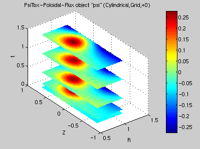
psi = psitbxtcv(10000,'+0')
 psi is a PsiTbx-Poloidal-Flux object =
       format: '+0'
         rmag: []
         zmag: []
    psitbxfun: [28x65x46 psitbxfun]
         iter: 10
          tol: 1.0000e-04
plot(psi)